Equations for the Gray Scott model can be found at:
https://groups.csail.mit.edu/mac/projects/amorphous/GrayScott/
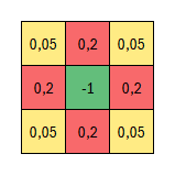
The Laplacian is done with a 2D convolution, using weights of 0.2 for adjacent cells and 0.05 for corners. Note that the sum of all elements for the convolution sum up 0.
The magma colormap, by Ander Biguri, is part of a set that can be downloaded from Matlab Central:
https://www.mathworks.com/matlabcentral/fileexchange/51986-perceptually-uniform-colormaps
Code:
% Reaction-Diffusion equation clc; clear; closeall; [X,Y] = meshgrid(linspace(-5,5,400)); A = ones(size(X)); B = zeros(size(X));% REaction starts full of A and with no B. But if so, reaction will not take place! % Add some droplets of B R = 0.5;% Radius of the droplets B(sqrt(X.^2+Y.^2)<R^2)=1;% 1st droplet, centered at origin B(sqrt((X-2*R).^2+(Y-2*R).^2)<R^2)=1;% 2nd droplet, centered at 2R,2R A = 1-B;% parameters Da = 1;% Diffusion rate for A Db = 0.5;% Diffusion rate for B dt = 0.1;% time step f = 0.02;% Feed rate for A. Will be scaled by (1-A) to prevent A>1 k = 0.05;% Kill rate for B. Will be scaled by B and added to f to prevent B<0 figure('color','k','menubar','none','ToolBar','none','NumberTitle','off'); I = imagesc(B); colormap(magma); axisequal off; for frame=1:10000 for i=1:50 An = A + (Da*Lapl(A)-A.*B.^2+f*(1-A))*dt; B = B + (Db*Lapl(B)+A.*B.^2-(f+k)*B)*dt; A = An; end set(I,'cdata',B); drawnow; end function z = Lapl(x) M = [0.05 0.2 0.05; 0.2 -1 0.2; 0.05 0.2 0.05]; z = conv2(x,M,'same'); end